
Suppose take a transfer function
G(S) H(S)= 10/(S+1)
To plot a Bode Plot for this Transfer function.
Open Matlab .
In the command window, write the co-efficients of S^2 and S as well as constant.
Following this rule, we shall write the numerator of G(S) H(S) as num=[0 0 10] , which means numerator only contains a constant i.e 10 .S^2 and S are absent
Coming to the denominator of G(S) H(S)=[0 1 1], which means denominator doesn't contains S^2, and co-efficient of S is 1 and the constant is 1.
Bode plot of above TF can be drawn in Matlab using matlab command Bode(num,den) as shown above.
Bode Plot :
G(S) H(S)= 10/(S+1)
To plot a Bode Plot for this Transfer function.
Open Matlab .
In the command window, write the co-efficients of S^2 and S as well as constant.
Following this rule, we shall write the numerator of G(S) H(S) as num=[0 0 10] , which means numerator only contains a constant i.e 10 .S^2 and S are absent
Coming to the denominator of G(S) H(S)=[0 1 1], which means denominator doesn't contains S^2, and co-efficient of S is 1 and the constant is 1.
 |
| Figure 1 |
Bode plot of above TF can be drawn in Matlab using matlab command Bode(num,den) as shown above.
Bode Plot :
 |
| Figure 2 |
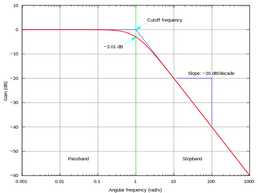
The transfer function G(S) H(S)=10/S+1 is a Single Pole transfer function.
Here cutoff Frequency wc=1/(coefficient of S) is 1 rad/sec.
As you all know actual bode plot differs from the approximation bode plot by -3dB as shown below
 |
| Figure 3 |
REFER TO FIGURE 2
We can see that, at the cut-off frequency or at the POLE, the Magnitude plot at the pole location varies by -3dB i.e (20dB-3dB=17 dB. Hence We can conclude that Matlab gives actual Bode plot.
Feel free to ask any questions. We shall see few more Transfer functions in the next post.